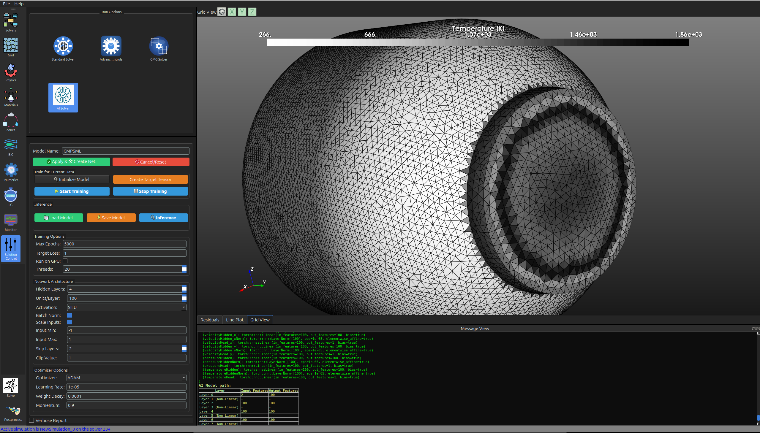
NeuralFlow

NeuralFlow verwendet neuronale Netze innerhalb einer vollständig konservativen Formulierung, anstatt sich auf die traditionelle PINN-Residualminimierung zu stützen.

Motivation

NeuralFlow ist ein CFD-Solver der nächsten Generation, der künstliche Intelligenz nutzt, um Strömungssimulationen zu verbessern und zu beschleunigen. Herkömmliche Solver diskretisieren und iterieren die zugrunde liegenden partiellen Differentialgleichungen (PDEs). Obwohl diese Methoden effektiv sind, können sie bei komplexen Geometrien oder hochpräzisen Turbulenzmodellen extrem zeitaufwendig sein.

Durch die Einbindung eines physikalisch fundierten neuronalen Netzes integriert NeuralFlow Domänenwissen direkt in den Lernprozess. Anstatt ausschließlich mit Daten zu trainieren, minimiert das neuronale Netz ein PDE-Residuum (oder einen Fluss) zusammen mit allen verfügbaren Simulationsdaten. Dies führt zu physikalisch konsistenten Lösungen, die schneller konvergieren als rein datengetriebene Ansätze.

Methodik

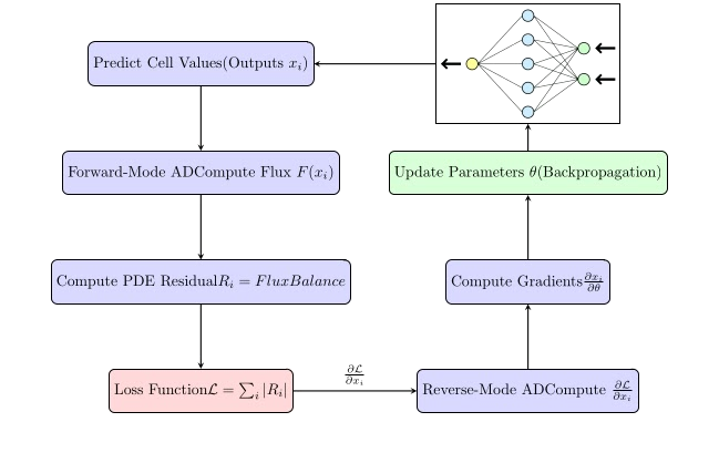
NeuralFlow nutzt zwei Formen der automatischen Differenzierung (AD), um das neuronale Netzwerk mit unserem CFD-Solver zu koppeln:

  • AD im Vorwärtsmodus: Wird bei den Fluss-/Residualberechnungen verwendet und erfasst partielle Ableitungen in Bezug auf die Ausgaben des neuronalen Netzes.
  • AD im umgekehrten Modus: Wird innerhalb des neuronalen Netzes selbst angewendet und ermöglicht Parameteraktualisierungen auf Basis der Rückpropagation mittels Kettenregel.

Dieser duale AD-Ansatz ermöglicht das durchgängige Lernen der Fluiddynamik: Jede Iteration treibt das neuronale Netzwerk an, Feldvariablen (z. B. Geschwindigkeit oder Korrekturfaktoren) zu erzeugen, die das PDE-Residuum innerhalb des Lösers minimieren.

NeuralFlow vs. klassische PINNs: Robustes physikbasiertes Lernen für reale CFD

Klassische PINNs

Ein auf klassischer Physik basierendes neuronales Netzwerk verwendet Differentialgleichungen direkt in seiner Verlustfunktion. Das Netzwerk muss die Ableitungen von Masse, Impuls und Energie an jedem Punkt exakt bestimmen. Dies funktioniert bei gleichmäßigen Strömungen, stößt aber bei Stoßwellen, Grenzschichten oder steilen Gradienten an seine Grenzen. In diesen Bereichen werden die Ableitungen groß oder undefiniert, was während des Trainings zu Instabilität und Oszillationen führt.

NeuralFlow

NeuralFlow verwendet stattdessen die Integralform (schwache Form) dieser Gleichungen. Das Netzwerk wird angewiesen, den Gesamtfluss durch jede Kontrollvolumenfläche zu minimieren . Diese Flüsse stammen aus fortgeschrittenen numerischen Flussberechnungsverfahren – wie AUSM⁺-up – , die in realen CFD-Solvern eingesetzt werden. Während des Trainings verwendet NeuralFlow die exakten Jacobimatrizen (Flussableitungen) des Solvers, wodurch Genauigkeit und Stabilität auch in der Nähe von Stoßwellen und dünnen Grenzschichten gewährleistet werden.

Warum es wichtig ist

  • Exakte Erhaltung: Flussbasierte Verluste gewährleisten, dass Masse, Impuls und Energie exakt erhalten bleiben.
  • Stoßwellen- und Grenzschichterfassung: NeuralFlow übernimmt direkt die Stoßwellenerfassungs- und Grenzschichtauflösungsfähigkeiten bewährter CFD-Numerikflüsse.
  • Stabiles und schnelles Training: Vom Solver bereitgestellte exakte Jacobimatrizen beschleunigen Konvergenz und Stabilität.
  • Effiziente Inferenz: Trainierte Netzwerke arbeiten mit der Geschwindigkeit neuronaler Netze, jedoch mit einer Genauigkeit auf CFD-Niveau.

Kurz gesagt, klassische PINNs differenzieren Gleichungen und stoßen bei Stoßwellen und Grenzschichten an ihre Grenzen. NeuralFlow integriert Flüsse, verwendet lösungserprobte numerische Flüsse und Jacobimatrizen und bleibt auch in anspruchsvollen Strömungsbereichen stabil und genau.

Mathematical Framework of NeuralFlow

Mathematical Framework of NeuralFlow

NeuralFlow is a next-generation CFD solver that combines advanced finite-volume methods with artificial intelligence to accelerate fluid simulations. Instead of replacing the CFD solver, NeuralFlow uses a Graph Neural Operator as a trainable correction engine. Starting from a CFD state, the neural operator performs several rollout correction steps on velocity, pressure, and temperature, with the objective of reaching a physically consistent solution in far fewer steps than a conventional solver iteration history.

Finite-Volume Conservation Form

Classical physics-informed neural networks usually enforce the pointwise differential form of the governing equations. This can be difficult for real CFD flows containing shocks, thin boundary layers, steep gradients, or discontinuities.

NeuralFlow instead works with the integral finite-volume form of the conservation laws. For each control volume, the solver measures the net conservation imbalance through the surrounding faces.

\( \mathcal{B}_i(V) = \sum_{f \in \partial \Omega_i} \mathcal{F}_f(V) A_f - S_i(V)\Omega_i = 0 \)

Here, \( \mathcal{B}_i(V) \) is the conservation imbalance of cell \( i \), \( \mathcal{F}_f(V) \) is the numerical flux through face \( f \), \( A_f \) is the face area, \( S_i(V) \) is the source term, and \( \Omega_i \) is the control-volume size.

This formulation directly enforces conservation of mass, momentum, and energy in the same way as a real CFD solver.

Graph Neural Operator Correction

The neural model does not directly replace the CFD solution. Instead, it predicts corrections to the current flow state.

\( V^{k+1} = V^k + \Delta V_\theta^k \)

where \( V^k \) is the current state and \( \Delta V_\theta^k \) is the correction proposed by the Graph Neural Operator. The correction is applied to the primitive flow variables, such as velocity, pressure, and temperature.

The purpose of the network is to learn a compressed convergence path. A classical implicit CFD solver may need many iterations to reach a converged state. NeuralFlow tries to learn how to reach a useful, physically consistent solution in only a small number of learned correction steps.

Multi-Rollout and Episode-Based Training

NeuralFlow uses multi-rollout correction. Starting from a fixed training state, the Graph Neural Operator applies several learned corrections in sequence:

\( V^0 \rightarrow V^1 \rightarrow V^2 \rightarrow \cdots \rightarrow V^m \)

After the rollout sequence, the CFD solver evaluates how well the final field satisfies the conservation laws.

Training is organized into episodes. Each episode starts from a fixed training anchor, performs a limited number of rollout/update steps, and then measures the true online conservation error at the end of the episode.

This gives the method a reinforcement-learning flavor. The CFD state acts as the environment, the neural operator proposes correction actions, and the conservation imbalance provides the physics-based feedback. However, the feedback is not a black-box reward. It is generated by an advanced implicit finite-volume CFD solver.

Learning from the Implicit Solver Methodology

The feedback used by NeuralFlow is not just a scalar residual value. It comes from the numerical methodology of the implicit CFD solver. The solver assembles the conservation imbalance and computes the sensitivity of the equations to the flow variables through flux Jacobians.

\( A = \frac{\partial \mathcal{B}}{\partial V} \)

This matrix contains the linearized finite-volume structure of the solver, including flux coupling, variable interactions, boundary-condition effects, and the sensitivity of the conservation equations to the solution state.

Therefore, the GNO learns not only from conservation laws, but also from the proven numerical structure of an advanced implicit CFD method.

Physics Loss and Solver-Guided Gradient

A physics-based objective can be written as:

\( \mathcal{J}_{phys}(V) = \frac{1}{2} \mathcal{B}(V)^T W \mathcal{B}(V) \)

where \( W \) is a weighting operator used to scale or emphasize different parts of the conservation imbalance.

The gradient with respect to the flow state is obtained through the solver's linearized system:

\( \frac{\partial \mathcal{J}_{phys}}{\partial V} = A^T W \mathcal{B}(V) \)

This is the key connection between the CFD solver and the neural network. The solver provides the physics-based direction in solution space, and the neural network learns parameters that generate better correction steps.

Dual Automatic Differentiation

NeuralFlow uses two forms of automatic differentiation.

Forward-mode automatic differentiation is used inside the CFD solver to compute flux Jacobians and the sensitivity of the conservation equations with respect to the predicted flow variables.

Reverse-mode automatic differentiation is used inside the neural network to update its trainable parameters through backpropagation.

\( \frac{\partial \mathcal{J}_{phys}}{\partial \theta} = \frac{\partial \mathcal{J}_{phys}}{\partial V} \frac{\partial V}{\partial \theta} \)

This dual-AD strategy allows NeuralFlow to combine CFD-grade flux linearization with neural-network training. The solver computes how the conservation equations respond to the flow state, and the neural network learns how to produce corrections that reduce the conservation imbalance more efficiently.

Memory-Efficient Episode Learning

Backpropagating through a long sequence of learned CFD corrections would require storing many intermediate graph states, messages, tensors, flow fields, and solver quantities. For realistic finite-volume meshes, this memory cost can become too high.

Episode-based training controls this cost by using short rollout windows. The model learns from the physics feedback over a limited episode, and the true online conservation error is measured at the end of the episode.

This makes the method practical for large CFD problems while still allowing the GNO to learn accelerated convergence behavior.

NeuralFlow Compared with Classical PINNs

Classical PINNs differentiate the governing equations directly and enforce the pointwise PDE form. This can become fragile near shocks, discontinuities, and thin boundary layers.

NeuralFlow instead integrates fluxes over control volumes. It uses solver-proven numerical flux methods, such as AUSM-type fluxes, and trains with solver-computed Jacobians. This gives the method the robustness of finite-volume CFD while retaining the learning capability of neural operators.

Conclusion

NeuralFlow is designed to learn a compressed convergence path for CFD simulations. It does not replace the governing equations or the CFD solver methodology. Instead, it uses a Graph Neural Operator as a trainable correction engine guided by conservation laws, finite-volume fluxes, exact solver Jacobians, and implicit CFD linearization.

The goal is to reach physically consistent CFD solutions in far fewer steps, while preserving the conservation, robustness, and numerical knowledge of advanced CFD solvers.

Was wurde bisher abgeschlossen?
✓ AD-Integration im Vorwärtsmodus für Flussberechnungen.
✓ Implementierung robuster neuronaler Netzwerkarchitekturen in C++ (LibTorch) für das In-Solver-Training.
✓ Einbeziehung von Randbedingungen und zusätzlichen physikalischen Nebenbedingungen (z. B. Energiegleichung) direkt in die Trainingsschleife.
✓ Nachgewiesene Effizienz bei kompressiblen Hochgeschwindigkeitsströmungen.

Zukunftspläne & Erwartungen
NeuralFlow befindet sich derzeit in aktiver Entwicklung, und wir erwarten Folgendes:

  • GUI-Integration
  • Multiphysikalische Integration
  • Transiente Probleme

In der nächsten Phase wollen wir Vergleichswerte mit herkömmlichen CFD-Solvern liefern, wobei der Fokus auf der Konvergenzgeschwindigkeit und der physikalischen Genauigkeit in komplexen Strömungsregimen liegt.